Runaway Wagons

Adrian Glasser – Land of Iron volunteer

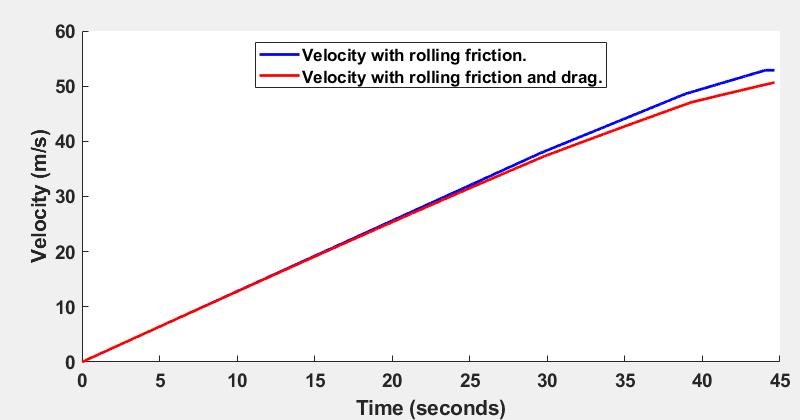
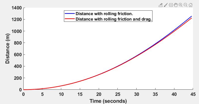
This blog describes calculating the velocity of runaway ironstone wagons as they careened down Ingleby Incline when a cable snapped. To cut to the chase, without friction and wind resistance, the wagons would have reached a velocity of 154 mph, but more realistically, with friction and wind resistance taken into account they would have reached about 113.36 mph at the bottom of Ingleby Incline in about 44.65 seconds.

For reference to the map below, the bottom of Ingleby Incline starts on the branch of the path going off towards the bottom right of the section of map. Click on the '-' button to see the full extent of Ingleby Incline to the moor top.

Location of Ingleby Incline.

Grid Reference: NZ 60025 03478

Latitude, Longitude: 54.4232, -1.0764

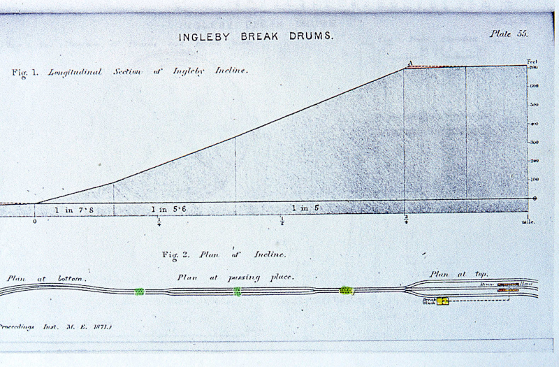
Ingleby Incline is located about three miles from Battersby Junction and extends up the North York Moors escarpment. Today it is a lovely, but steep, footpath up the hill with wonderful views from the top. It used to be the site of an industrial railway where ironstone was brought down from the ironstone mines on the moors to the railways that carried it to the smelting kilns in Durham and beyond. The railway up Ingleby Incline was built in 1860 and consisted of a double set of tracks. From Incline Foot at the bottom, with a gradient of about 1 in 11, to Incline Top with a gradient of 1 in 5, the incline extends 1430 yards (1307.6 meters) to the moor top. Wagons loaded with ironstone, were lowered down the incline on steel cables 1650 yards long that went around a 14 ft break drum in the stone-built Drum House at Incline Top. The ironstone laden wagons were lowered, three at a time, while empty wagons or wagons filled with coal were pulled up the incline to partially counterbalance the weight on the adjacent tracks. It would normally have taken about 3 minutes for the loaded wagons to be lowered down at about 20 miles per hour.

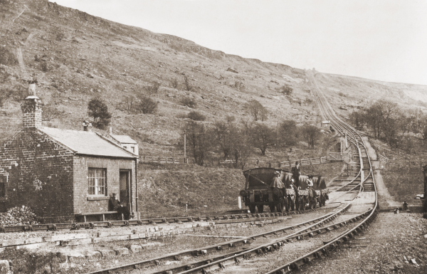
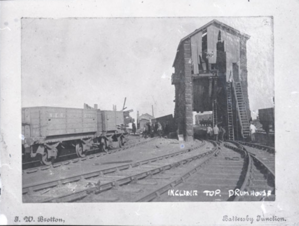
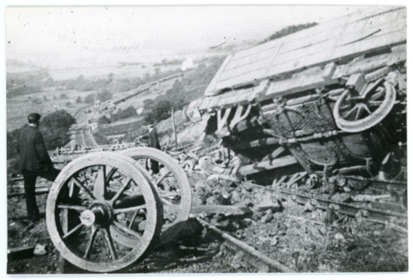
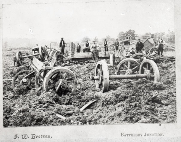
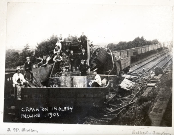
Occasionally, disaster struck when the cable snapped under the 50-ton weight of the loaded wagons full of ironstone and the wagons careened down the incline, either flying off the rails or smashing into stationary wagons on the tracks at Incline Foot. Although there were catch-points on the rails near the top and bottom to direct runaway wagons off the tracks, the wagons were not always successfully diverted off the main tracks to the safety of these catch-points. There are numerous old photographs of the carnage caused by these incidents and runaway wagons with smashed wagons, wagon wheels and piles of spilt ironstone beside the tracks. Old photographs also show the damage to the break house at the top caused by the tremendous whiplash from the tension released in the cable when it snapped. These dramatic incidents would have been memorable for the sheer terror caused by the snapped cable and the speed of the loaded wagons and the force and ferocity of their impact on anything in their way.

These photographs are courtesy of Ryedale Folk Museum and Beck Isle Museum archive and where noted on the photographs are photographed by T. W. Brotton. The photographs are thought to date from 1903.

Ingleby Break House — Damage from a Snapped Cable to Drum House

Tom, the Land of Iron Programme Manager, asked if it might be possible to calculate the speed reached at Incline Foot by a fully loaded set of runaway wagons from a snapped cable at Incline Top. There are good records of the length of Ingleby Incline and the gradients down the incline and with a few assumptions, it is possible to calculate the velocity. I did some initial calculations with some simplifications and assumptions;

Weight of the loaded ironstone wagons: 50 T
Distance down the incline ($d$): 1225 meters
Acceleration due to gravity ($g)$: 9.8 m/s²
Kinetic (i.e. moving) friction of the loaded wagons: 0
Initial velocity ($vi$) of the wagons at Incline Top: 0 m/s
Gradient of the incline: 1 in 5

If friction is neglect, the following equations can be used:
To find the final velocity (vf):
$$ {vf^2 – vi^2 = 2*a*d} $$
where $vf$ is final velocity, $vi$ is initial velocity, $a$ is the acceleration and $d$ is distance. This equation requires knowing the acceleration of the wagons and we can calculate the acceleration from:
$$ {a = g * sin(theta) } $$
where $a$ is the acceleration down a slope, $g$ is the acceleration due to gravity and $theta$ is the angle of the gradient in degrees.

Notice, that in assuming no friction, acceleration due to gravity is constant and the acceleration of the wagons depends only on the gravitational force and the angle of the slope. The weight of the wagons is not actually used in this calculation.

A gradient of 1 in 5 means a 1 m rise for a 5 m run. From this we can calculate the angle of the gradient in degrees.

From: $$ {tan(theta) = opposite/adjacent} $$

the angle of the incline can be calculated to be: $$ {theta = arctan(opposite/adjacent) = arctan(1/5) = 11.31 \quad degrees} $$ Then from: $$ {a = g * sin(theta)} $$ the acceleration of the wagons can be calculated to be: $$ {a = 9.8 * sin(11.31) = 1.922 \quad m/s^2} $$ Then from: $$ {vf^2 – vi^2 = 2*a*d} $$ the final velocity can be calculated to be: $$ {vf = \sqrt(2*a*d +vi^2) = \sqrt(2*1.922*1225 + 0^2) = 68.62 \quad m/s} $$

$$ {68.62 \quad m/s \quad is \quad 247.04 \quad km/hour \quad or \quad 153.5 \quad mph} $$

Having calculated the acceleration and knowing the mass of the wagons (50,000 kg), the force generated by the accelerating wagons can be calculated to be:

From: $$ {F = m * a = 96,100 \quad Newtons} $$

I presented this information to Tom and he shared it with some of the Land of Iron aficionados and one commented,

"Ah, yes, but what about the wind resistance of the wagons as they accelerated down Ingleby Incline. The resistance increases with the square of the velocity."

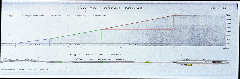
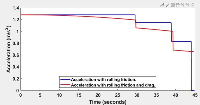
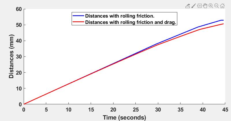
Further, the historical details of Ingleby Incline indicate that it was not a constant gradient of 1 in 5, but actually composed of three sections with three different gradients. So, could that be incorporated into the calculation? Further, the assumption of zero kinetic friction is not accurate, so could the friction be incorporated too? Kinetic friction is the friction when the wagons are moving. That would be the friction of the wheels on the tracks, of the wheels on the axles and on any bearings. Well, of course, with some assumptions and simplifications, it is possible to calculate the final velocity incorporating these factors too. However, this becomes somewhat more complicated because if the wind resistance is changing with the square of the velocity, then this means that as the wagons accelerate down the incline and the velocity increases, so too does the wind resistance and this then decreases the acceleration and so it reduces the velocity. This is a situation where something changes as a function of something else that changes. This is exactly what calculus is used for.

There is another way to calculate something like this without resorting to calculus and that is to use a computer program. Computer programs are good because they do exactly what they are told to do (but this also means they are bad if they are told to do something wrong), but they are also good because they can do repeated calculations over and over again and generally don’t complain about doing that.

The way to use a program to do these calculations is to do the calculations over and over again for very small increments. In computer programming this is called a loop. A loop is where the same calculation is repeated over and over again and the values at the end of the calculation on the previous iteration through the loop are passed to the start of the loop in the next iteration. As the wagons move down the incline, the time changes and the distance the wagons move down the incline change progressively. So, the program could do a loop around very small distance increments down the incline or the program could do a loop around very small time increments. For this particular calculation, it turns out that the best way to do this is as a function of time because at each time interval, the acceleration can be calculated, then the velocity can be calculated, then the drag (the resistance from wind resistance) can be calculated, then the new acceleration as slowed by the drag can be calculated and then the new velocity with the acceleration affected by drag can be calculated. If the new velocity is known at each time interval, the distance travelled over the time interval at that velocity can be calculated. So, by setting the time intervals to be something very small, like 0.001 seconds, these calculations can be performed over and over again as the wagons careen down the incline, adjusting the drag, the acceleration and the velocity at each new time interval, and calculating the distance travelled at each time interval. The assumption that is made in using a loop to do this in very small time increments is that the velocity is constant for each time increment. This is not true when acceleration is changing, but the smaller the time increments, the more accurate is this assumption.

In using a computer program to do this, the time intervals could be made even smaller if needed, all that means is the entire calculation would take a little longer and there would be more iterations. If these calculations were to be done, then it is of interest to know how the acceleration, the velocity, the drag and the distances moved are changing as the wagons careen down the incline. Knowing these things would be interesting to see and they would be helpful for understanding if the calculations are correct, or if something goes wrong along the way. We can look at these numbers by plotting graphs of these numbers as a function of time. Further, if doing these calculations, the results with drag could be compared to the results calculated without drag. This would help to understand what the effects of the drag are. So, to be able to show all these results means that the numbers calculated at each time interval should be stored so they can be plotted when the calculations are completed. This adds one other consideration as to the appropriate time interval to choose, and that is, if very small time increments are used there will be many of them, so all the numbers from all the calculations at all the different time points will have to be stored and this increases the amount of memory that the program must use to perform these calculations and it affects how much data is available at the end of the calculations to display. The computations and the memory required for these calculations won’t be demanding on a computer program because programs can do far more demanding tasks than this, but to keep it reasonably simple, it would be better not to use too small a time increment. There are some other considerations as to what time interval to use. The iterative calculations assume that acceleration is constant at each time interval. This is not in fact correct as acceleration is constantly increasing (and changing with drag) even during each time interval. This does add some inaccuracies that calculus does not suffer from, but, so long as the time intervals are small enough, the inaccuracies caused by this compared to what would be calculated with calculus, will be acceptable.

There are, in fact, many inaccuracies in these calculations, because it is not possible to know the true friction of the wagons and it is not possible to know the true drag from wind resistance. Wind resistance is affected by the turbulence of the air flow over the wagons, how long the line of wagons is, how aerodynamic (or not) the wagon are, etc. It is virtually impossible to know all these details and many of them would have to be established by doing actual testing with scale models to know them more accurately.

The programming language I have chosen to do these calculations in is Matlab because it is the programming language I have most experience with and I know it better than I know the several other programming languages I use from time to time. A programming language is just like a language in many ways. The more one knows it, the more fluently one can speak it and the more elegant one’s conversations are. It's just the same with a program. The better you know a programming language, the better the program will be. There are many freely available programming languages like Python or Processing, for example. They would work perfectly well too.

An engineering image of Ingleby Incline exists which shows the gradients, the distances and the overall heights of Ingleby Incline. It is useful and a valuable resource, but the image suffers from the disadvantages that it is not perfectly horizontally oriented and the horizontal and vertical axes are not the same scale.

Ingleby incline diagram — Ingleby Incline Engineering Diagram

The image can readily be rotated to get it perfectly horizontal. That the horizontal and vertical scales are different is of no concern if all one wants to do is to look at the image, but it is unfortunate if one might want to do some more accurate measurements from the image. There is a way to fix this and that is to rescale the image so that the horizontal and vertical scales are the same. Fortunately, the image does have both a vertical and a horizontal scale on it. From these, the horizontal and vertical scale factors can readily be calculated in image pixels per unit distance shown on the image (miles for the horizontal and feet for the vertical). The computer program comes in handy here too because the program can be readily written to load, rotate and rescale the image correctly, providing that the scale factors are known. It is easy to get the scale factors by measuring the horizontal and vertical distances and the horizontal and vertical numbers of pixels in the image that span those distances. With that information, the image can be rescaled and then when rescaled, all the distances can be measured directly from the image in pixels and then converted to actual distances. This was done and all the distances used in the calculations come from the rescaled image. In addition, the three different sections of Ingleby Incline with different gradients are marked as triangles of blue (bottom), green (middle) and red (top). The distances along each of the gradients can then also be calculated directly from the rescaled image using the Pythagorean theorem that states that in a right-angled triangle the square of the hypotenuse is equal to the sum of the squares of the two other sides.

Ingleby incline diagram scaled — Scaled and Rotated Ingleby Incline Engineering Diagram

The calculations were repeated with rolling friction introduced. It turns out this is relatively easy to do. All one has to do is to calculate the acceleration using: $$ {a = 2/3*g * sin(theta)} $$ for rolling friction versus: $$ {a = g * sin(theta)} $$ for frictionless sliding.

Since a program was being used to do the calculations, it is readily possible to do the calculations both with and without drag, that is the resistance due to air. This allows for a nice comparison as to how drag affects acceleration and velocity. In all the following graphs, the results with (in red) and without (in blue) drag are shown.

The calculations for the effect of drag are based on the following equation: $$ {F_d = -1/2*p*A*C_d*|v|^2} $$ Where $F_d$ is drag force in units of $N/(m^2)$, $p$ is the density of air which typically has a value around 1.2 $kg/m^3$ - although this depends on air temperature and altitude, for example. $A$ is the cross-sectional area of the front of the wagons, $v$ is the velocity and $C_d$ is the unitless drag coefficient which depends on the shape of the object (the wagons in this case). For a spherical object, a value of 0.47 is typical. I found a value for trains of 1.02 from a publication by S. Watkins, J.W. Saunders and H. Kumar. Aerodynamic drag reduction of goods trains. Journal of Wind Engineering and Industrial Aerodynamics, 40 (1992) 147-178. Obviously, there are many other factors that can affect drag, including if the air is not still and if not, what direction the wind is blowing, the shape of the wagons, how aerodynamic they are, etc.

Notice that the drag equation uses the magnitude of the velocity squared. The faster the wagons go, the greater the air resistance. I got the approximate area of the front of the first wagon from Tom Mutton to be 2 m x 2.5 m.

Wikipedia has a useful section on drag coefficients.

Newton's second law of motion: $$ {F = m * a} $$

will be used, but here we are actually calculating a deceleration, not an acceleration because the drag slows down the acceleration. So, here, just for the moment, the acceleration above will be referred to as deceleration ($D_a$). $$ {F_d = -1/2 * p * A * C_d * v^2 = m * D_a} $$ then, rearranging that equation gives: $$ {D_a = (-1/2 * p * A * C_d * v^2)/m} $$

So, to calculate the acceleration adjusted for drag, one must first calculate the acceleration without drag, then calculate the acceleration adjusted by drag and subtract the latter from the former. That gives the following equation: $$ {a_d = a - (1/2 * p * A * C_d * v^2)/m} $$ where $a_d$ is the acceleration adjusted for the drag and $a$ is the acceleration calculated without drag. This calculation is performed over and over again for each time interval during the loop and then from this calculated acceleration adjusted for drag, the velocity and the distance travelled can be calculated at each new time interval.

Velocity is calculated as acceleration multiplied by time. From looking at the units, it is possible to check this relationship because acceleration in units of $m/s^2$ multiplied by time in units of seconds gives $m/s$, which are the units for velocity. The final velocity ($v_{fd}$) at each time interval is calculated as the sum of the velocity calculated at the previous interval ($v_{id}$) plus the change in velocity due to the new acceleration including drag ($a_d * dt$): $$ {v_{fd} = v_{id} + a_d * dt} $$ The distance travelled ($d$) during the time interval is given by the initial velocity ($vi$) plus the average of the new velocity during the time interval ($dv/2$) multiplied by the time interval ($dt$): $$ {d = (vi + dv/2)*dt} $$ Again, this can be checked with the units. Velocity is in $m/s$ and velocity multiplied by time in seconds gives the distance in meters. Since the acceleration was calculated, the equation for distance shown above can be expanded and expressed using the acceleration which gives: $$ {d_{fd} = d_{id} + (v_{fd} * dt + 1/2 * a_d * dt^2)} $$ where $d_{fd}$ is the final distance with drag, $d_{id}$ is the initial distance with drag, $v_{fd}$ is the final velocity with drag, $dt$ is the time interval, and $a_d$ is the acceleration with drag.

The way the calculations are performed is that for each time interval, the values of interest are stored so that once all the calculations are completed, the values of interest can be plotted to show how various things change with the time increments. The acceleration, velocity and distance travelled at each time interval are all stored during the loop and are plotted as a function of time at the end of the calculations in the graphs shown below.

The resulting graph of acceleration versus time initially looks a bit odd, but that's because the incline has three sections each with a different gradient. The calculations for acceleration are based on the slope of the gradient, so when the gradient changes, the acceleration changes instantaneously in the calculations, decreasing for flatter slopes. In the real world, the acceleration would change gradually as the wagons went from one gradient to another, so the calculations are inaccurate because of this. Because acceleration decrease instantaneously in the calculations, but would decrease gradually in the real world, this means that the calculations actually underestimate the actual final velocity. It is clear that as the runaway wagons head downhill, the acceleration decreases at each flatter gradient, and with drag from air resistance (red line), the acceleration decreases even further. The acceleration curve for the wagons without drag (blue line) drops below that of the red red line at the end because the wagons without drag move faster, so they reach the bottom of the incline which is flat, before the wagons with drag. Naturally, the calculations have to proceed until the wagons with drag reach the end.

graph acceleration vs time — Graph of Acceleration vs Time

The graph of velocity as a function of time also shows the different velocities for the three different gradients, but the differences are not quite so obvious. As expected, the velocity is slower for the wagons when the drag is considered (red line). After 44.647 seconds, the velocity of the wagons with drag reach 113.36 mph. At the very end, the wagons without drag reach the end of the incline before the wagons with drag (there is a very small horizontal line at the end of the blue line). This indicates that the wagons without drag have reached the bottom of the incline where the velocity would be constant or slowing down.

graph velocity vs time — Graph of Velocity vs Time

The graph of distance as a function of time progressively increases until the wagons reach the end of the incline, although the distance reached at the end is slightly less for the wagons with drag than for the wagons without drag.

graph distance vs time — Graph of Distance vs Time

This last graph, below, shows the distances travelled for the wagons for each tiny time increment of the programming loop. This is really a test to see how fine the time and distance increments in the calculation are. The incremental distances really are in units of millimeters, meaning that the wagons move just a matter of a few millimeters for each 0.001 second time increments. Towards the end of the run as the wagons reach their maximum velocities, the wagons are still only travelling about 50 mm (5 cm) for each time increment. This is a pretty small distance and so the inaccuracies introduced by virtue of doing this calculation with a loop rather than with calculus are probably sufficiently small to not make an appreciable difference to the final outcome.

graph distances vs time — Graph of Distances Travelled vs Time

With the need for some assumptions, for it is impossible to know all the details with certainty, these calculations (if they are correct) show that the final velocity of the runaway ironstone wagons with rolling friction and drag due to air resistance would have reached 50.676 m/s or 113.36 mph after 44.647 seconds and the wagons would have reached a final acceleration of 0.659643 m/s² at the bottom of Ingleby Incline. That is quite a speed and with 50 tons of weight this would have resulted in a tremendous force at the bottom.